Algorithms From Scratch: Linear Regression

A linear regression model is the simplest of all machine learning models. In fact, calling it a machine learning model in the first place makes it sound more complicated than it really is. All we want to do is find a set of parameters(think slope and y-intercept) that properly relates an input to an output. When you got a scatter plot of points and drew a line of best fit through them, you were a linear regression model.

Those problems were typically in the form \(y=mx+b\). Here, \(m\) and \(b\) are the paremeters we want to learn, \(x\) is the input data, and \(y\) is what we’re trying to predict. This could be, for instance, for predicting someone’s weight based on their height.

For most projects, however, we want more than one input dimension. There could be many input features. Imagine you want to predict the price of the car using a linear model. For input, you might have the car’s age, brand, mpg, etc. To generalize the \(y=mx+b\) formula to higher dimensions, we have to use linear algebra.

The formula is \(Ax=b\). \(A\) (which includes a column of \(1\)s for the y-intercept term) is our input data, \(x\) is the parameters, and \(b\) is the output. It’s a little confusing since \(x\) and \(b\) were completely different before, but you should get used to this representation.

This problem would be really simple to solve for if \(A\) were invertible, since we could simply do:

Unfortunately, that requires that A is invertible, meaning that A must be a square matrix. This is essentially never the case for any dataset—have you ever seen a dataset with as many columns(features) as rows(individual data points)? So we need some way to find x without using the inverse.

SVD

The singular value decomposition factorizes a matrix \(A\) into three components: \(U, \Sigma,\) and \(V^{T}\).

This equation comes from \(AV=U\Sigma\). \(V\) is the right singular vector matrix, \(U\) is the left singular vector matrix, and \(\Sigma\) is the singular value matrix. At this point, you might notice that \(V\) was moved over to the other side of the equation just by finding the transpose. This is because both \(U\) and \(V\) are orthogonal matrices, meaning that \(V^{-1}=V^{T}\). But why is that the case? It comes back to how we get \(U\) and \(V\) in the first place: eigendecompositions.

An eigendecomposition factorizes a square matrix \(A\) into two matrices, one for the eigenvectors and the other for eigenvalues.

\(AV=V\Lambda\) or \(A=V\Lambda V^{-1}\)

When the matrix is symmetric, the eigenvectors will be orthogonal to eachother and therefore \(V^{-1}=V^{T}\).

Since \(U\) and \(V\) are both orthogonal matrices, there’s clearly some relation to the eigenvalue decomposition of a square and symmetric matrix. As it happens, we can transform our matrix A into a symmetric and square matrix by multiplying itself by the transpose —\(A^{T}A\). Plugging the SVD factorization back in for \(A\), we get this.

The same goes for U, except we right multiply the transpose.

Both \(U\) and \(V\) can be found by finding the eigendecomposition of the data matrix \(A\) multiplied by its transpose in different directions.

This is the basic concept of the SVD. While there’s a lot more to go into, that’s all we really need. Now that there’s a simple factorization for \(A\), we can find it’s pseudo-inverse and use that to solve the equation \(Ax=b\).

SVD Implementation

Although finding the singular value decomposition seems relatively simple, it’s difficult to implement. Instead, we’ll use the svd function from numpy.linalg. We’ll also import make_regression sklearn.datasets to create a simple dataset.

import numpy as np

from np.linalg import svd
from sklearn.datasets import make_regression

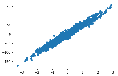
I want to start out on a dataset with 1000 samples and just one feature so it can be visualized easily. To account for the bias term, we have to add a column of zeros to \(A\). \(A\) now has the shape \((1000, 2)\).

A, b = make_regression(n_samples=1000, n_features=1, noise=10)
A = np.hstack((A, np.ones(shape=(A.shape[0],1))))

Now that the dataset is in order, let’s find the SVD of \(A\).

U,S,V_T=np.linalg.svd(A, full_matrices=False)
#svd returns S as a 1d-matrix, so we have to diagonalize it
S=np.diag(S)

np.allclose(A,U@S@V_T,atol=1e-10) #returns True -> U@S@V_T=A

The shapes of U,S, and V_T are (1000, 2), (2, 2), (2, 2). We’re not getting the full matrices because we want the economy SVD. The economy SVD truncates elements of the array that aren’t needed and puts it into a shape that we can multiply together. If full_matrices=True, U would have the shape (1000, 1000).

To get \(x\) like we wanted, all that’s left is to use that inverse SVD formula above.

inverse_SVD= (V_T.T@np.linalg.inv(S)@U.T)
x=inverse_SVD@b

x should be the shape (2,). The slope is the first term and the y-intercept is the second. Finding the corresponding output is as simple as taking the dot product of the parameters and the row vector of A. predict_mult just applies the prediction function to all of A.

def predict(parameters,x):
    return parameters@x

def predict_mult(parameters,x_array):
    predictions=[predict(parameters,x) for x in x_array]
    return predictions
  
y_pred=predict_mult(x,A)

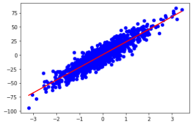
You can also test this process with a higher number of features(dimensions) and it’ll work properly. My mean squared error for the 2D example shown above was 100 and was 98 for 3 features.