The Timbre Problem

“Understanding timbre is perhaps the most challenging problem facing the musical community at the present time… Timbre is an area that is ripe for investigation, but certain methodological and conceptual problems arise.” - Carol L Krumhansl

That quote was written way back in 1989. Ten years later, Keith Dana Martin wrote that timbre “is empty of scientific meaning, and should be expunged from the vocabulary of hearing science.”

Twenty years later, scientists are still arguing about the exact same thing.

What is it?

First, we have to define timbre. This itself is a very contentious subject—here’s a list of different definitions— but generally people agree that timbre is the quality or character of an instrument, regardless of pitch, duration, and loudness.

For example, a piano and an oboe playing a C4 at the same volume will sound different. Timbre is what separates these two tones. As you can tell, it’s a really straightforward concept. Unfortunately, that’s also what makes it so frustrating since no one has succeeded at concretely describing what we can naturally hear.

It’s important to note that timbre is a perceptual quality, meaning that it’s based on a human’s recognition of sound. This subject is up for debate; physicalists argue that the entirety of timbre can be captured through a deeper understanding of the physical sound. Nevertheless, many studies treat timbre more as a perceptual aspect by using dissimilarity ratings in their analysis. The setup for dissmilarity ratings is as follows: “Two tones are presented in succession per experimental trial, and listeners rate their degree of dissimilarity, such that the task does not require any verbal labeling of sounds.” These ratings are often combined with mathematical scaling techniques to create a “latent space” of different timbres. John M. Grey created this timbre space in his 1977 paper “Multidimensionalperceptual scaling of musical timbres”:

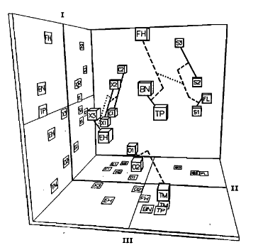
Imagine these cubes as different instruments. Their position in the space describes the timbre with respect to other instruments. At the bottom, O1(an oboe) is located close to O2(another oboe), meaning that these instruments are timbrally similar.

Researchers examine their respective spectral and temporal qualities in this timbre space to find similarities. This helps them define concrete spectral (frequency) and temporal (time) characteristics like the spectral centroid or ASDR that relate to an instrument’s timbre.

This is an excellent way of understanding the physical qualities of timbre, but what if it could be a continuous, regularized timbre space(we can find timbres for any mystery instrument in between the points), millions of trials could be ran, and it’ll all run without humans? Wouldn’t that be great?

Enter Autoencoders

Autoencoders are a neural network architecture composed of two parts. There’s an encoder and a decoder. The encoder receives input data, such as an image, and passes them through any number of layers into a significantly smaller representation. This smaller “bottleneck” is the latent space or latent embedding. The decoder takes the bottleneck as input and upscales it back into the original shape of the input. The goal of an autoencoder is to reconstruct the original input as accurately as possible.

The layers function similarly to any other neural network. There are convolutional autoencoders, sparse autoencoders, deep or shallow autoencoders, etc. A normal autoencoder also uses a loss function just like a regular NN to judge reconstruction.

Like many other deep learning projects, the MNIST dataset, consisting of 70,000 total handwritten digits, is a common starter for people looking to build an autoencoder.

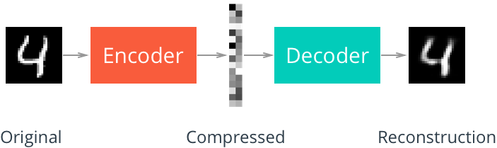
Here’s an example of an autoencoder reconstructing MNIST digits. As you can see, the latent embedding denoted with “Compressed” looks like random grayscale colors. Each pixel actually represents a weight. The top left pixel is black, meaning that it’s activated. That node in the latent space describes some feature of this “4” in a compressed format. It could be something like how the four loops around at the top, for example. What’s important to understand is that the latent space represents some component of the “4”, without actually describing any of the pixel values.

Here’s a view of the entire latent space: 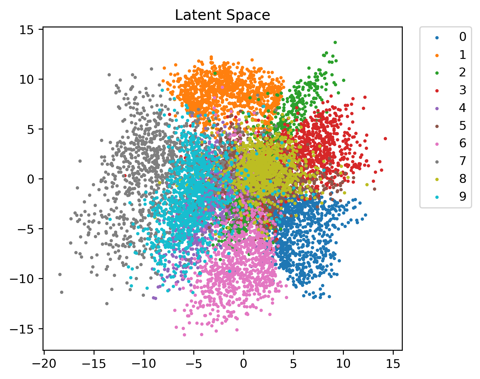As you can see, different locations in the space correspond to different numbers. Digits like 4 and 8, which look similar depending on the person’s handwriting, are close in the timbre space. Others, such as 1 and 6, are on opposite sides since they look nothing alike.

Getting Variational

Up until this point, I’ve described regular autoencoders. The latent space for autoencoders is not regularized, meaning that there isn’t information for certain points in the space. For certain applications, like denoising, this is fine. However, having a regularized distribution opens up a bunch of new possibilities, especially in generating new samples.

A variational autoencoder, instead of reducing to the latent space shown above, tries to learn a probability distribution for the input data. Instead of bottlenecking into one value, the encoder squeezes the input into a probability distribution. This is why VAEs are so closely related to Bayesian probability. The latent space has two separate components: the mean(or means for a multi-dimensional latent space) and standard deviation(s). The distribution is up to choice, but it’s common to use a Gaussian with mean 0 and standard deviation 1.

By learning a continuous distribution, we can sample anywhere from the latent space and get something that makes sense.

If you’re familiar with Bayesian probability, this section might help you understand the idea of variational inference. If not, then I’d recommend skipping it.

Variational Inference

First, I’m going to lay out some variables.

\(X\) = observed variables = our dataset

\(z\) = latent variables that we want to learn

The problem is that we don’t know $P(x)$. If you expand this distribution, you’ll find that its intractable.

Skipping a few steps of the derivation gives us…

\(\log{p(x)}\) is known as marginal-log likelihood. Rearranging in terms of this, we get.

While the KL-Divergence term is still intractable, there’s an important property to remember: it must be greater than or equal to 0.

The right term is known as Evidence-Lower Bound. By maximizing ELBO in this formula, we will minimize KL-Divergence. It’s a very clever solution that gives us an optimization problem.

Doing more rearranging gives the formula:

This bayesian view can be linked back to the original VAE architecture. The first term is the reconstruction error and the second is KL-Divergence, which is essentially finding a ratio of probability distributions.

From this perspective, the VAE structure seems pretty genius, right?

Using Audio in ML

In a perfect world, you could just pass a direct audio signal into a VAE and get a proper reconstruction. Unfortunately, it isn’t that easy.

Most architectures for deep learning are built around computer vision, so it’s much simpler to represent audio as an image.

Spectrograms

Normal audio – what’s sent to your speakers when you listen to music – is represented through a waveform in the time domain. It’s representing how air pressure changes in the air.

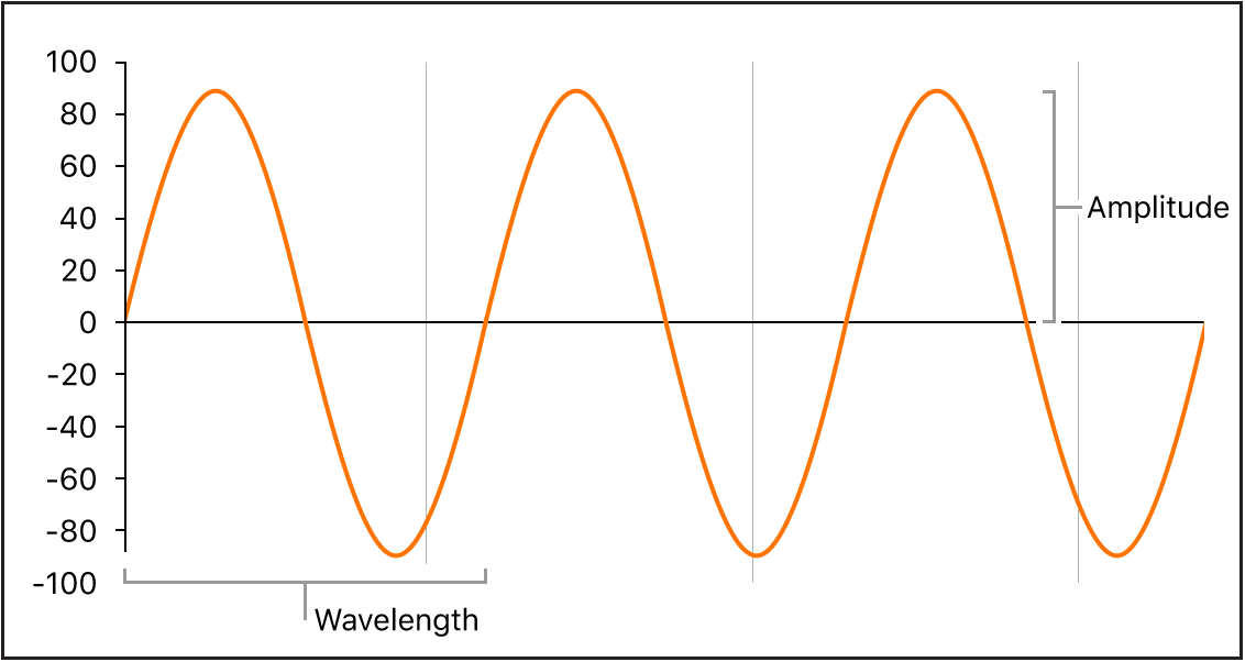
Tonal sounds are composed of periodic signals. The one shown above, for example, is a simple sine wave. More complex signals combine a series of sin waves. Using the Fourier transform, we can decompose a signal into the frequencies of the sine waves. The short-time Fourier transform, STFT, captures this series of frequencies at small snippets of time. By going through an audio signal and taking the STFT periodically, we can get a graph of frequencies over time. This is the basic idea of a spectrogram.

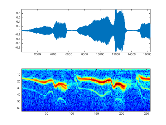
In this image, a 250ms audio signal is transformed into a spectrogram. Higher up translates to a higher pitch, and the redder the signal, the louder that frequency. As you can see, spectrograms are pretty intuitive.

The only issue with spectrograms is that you can’t play them; it has to be converted back to a waveform first. The reconstructed waveform can only be an approximation of the original since a spectrogram loses some key information, so you’ll never get great quality. There are ways to improve the reconstruction, but the quality will inevitably be lost.

Despite these drawbacks, spectrograms are the input of choice for most deep learning projects. Some models use Wavenet, a vocoder built out of diluted convolutional neural networks. In some cases, they can perform much better than Griffin-Lim reconstruction (the traditional inversion method) from a Mel-spectrogram.

Bringing It All Together

By combining VAEs and a proper dataset of spectrograms, we can, in theory, create a more interpretable timbre space that can be interpolated through. Putting aside the “timbre problem” for a second, there’s so many interesting opportunities for this to be used for music.

Imagine the perfect disentangled latent space. There would be three axes: the pitch, the loudness, and the timbre. It’ll almost certainly be more complex than this, but for a second act like timbre can be represented in a single dimension and all the axes are independent.

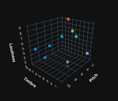
Then, you could load in a database of instrument notes and construct a latent space of instruments. Because its a VAE, you could interpolate between two instruments. It’d be the plugin to end all plugins.

From a scientific perspective, having a interpolable latent space would make it so much easier to investigate the physical sources of timbre. By slightly nudging along the piano-violin line and observing the differences in the resulting spectrogram, you could get a much better idea of what’s contributing to that difference. This is similar to what Grey was doing in the ’70s, but so much simpler. There’s no need for human dissimilarity ratings, and you can explore the latent space as thoroughly as possible.

Current Research

Because of the popularity of style transfer in computer vision, timbre transfer is a popular avenue to explore timbre. There are plenty of papers I could show here, but I specifically wanted to show the wide variety of modifications that can be applied to the traditional VAE architecture.

1. Timbre Transfer with VAE-GAN & WaveNet - This paper proposes a really interesting hybrid architecture that combines a VAE and a Generative-Adversarial Network(GAN). GANs are similar to VAEs in that they’re composed of two parts. A GAN differs because it uses a generator to create the input to the discriminator, which judges if the input is real or fake. In this architecture, the generator is a VAE. Wavenet is used to reconstruct audio and partially avoid phase issues(the problem with inverse STFT).
2. TimbreTron - In this paper, researchers once again make use of GANs. CycleGAN is an extension of regular GANs, using two generators and discriminators.

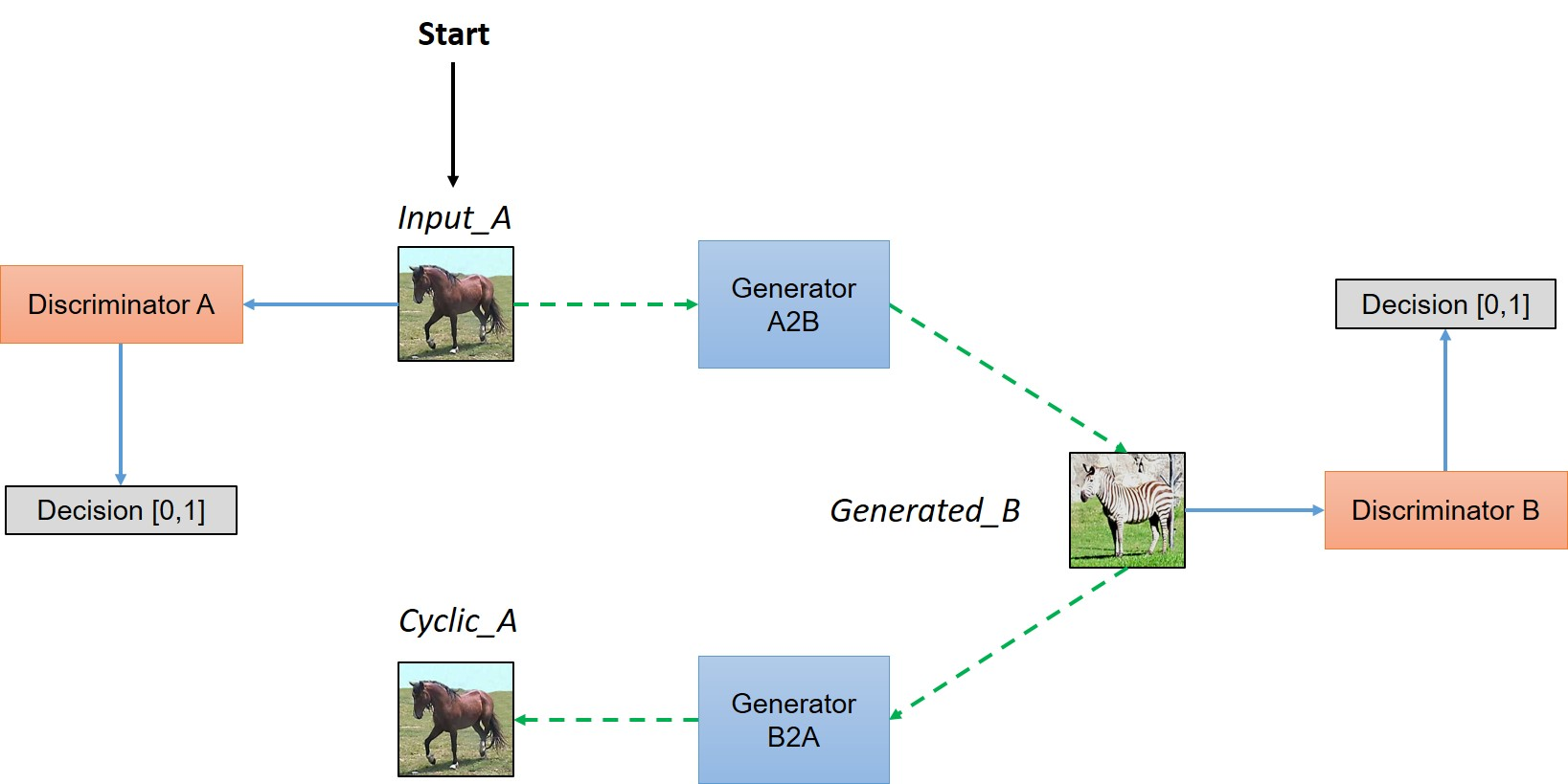
The output is passed into a WaveNet synthesizer to avoid ISTFT reconstruction issues. The Constant-Q Transform, CQT, is used in the place of the STFT since the researchers found it improved quality at certain ranges.

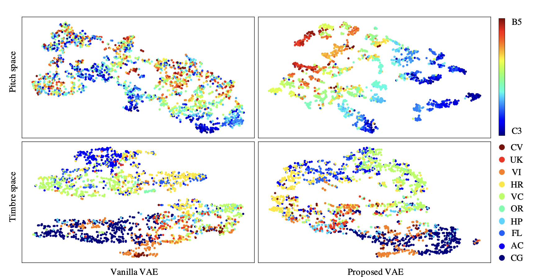
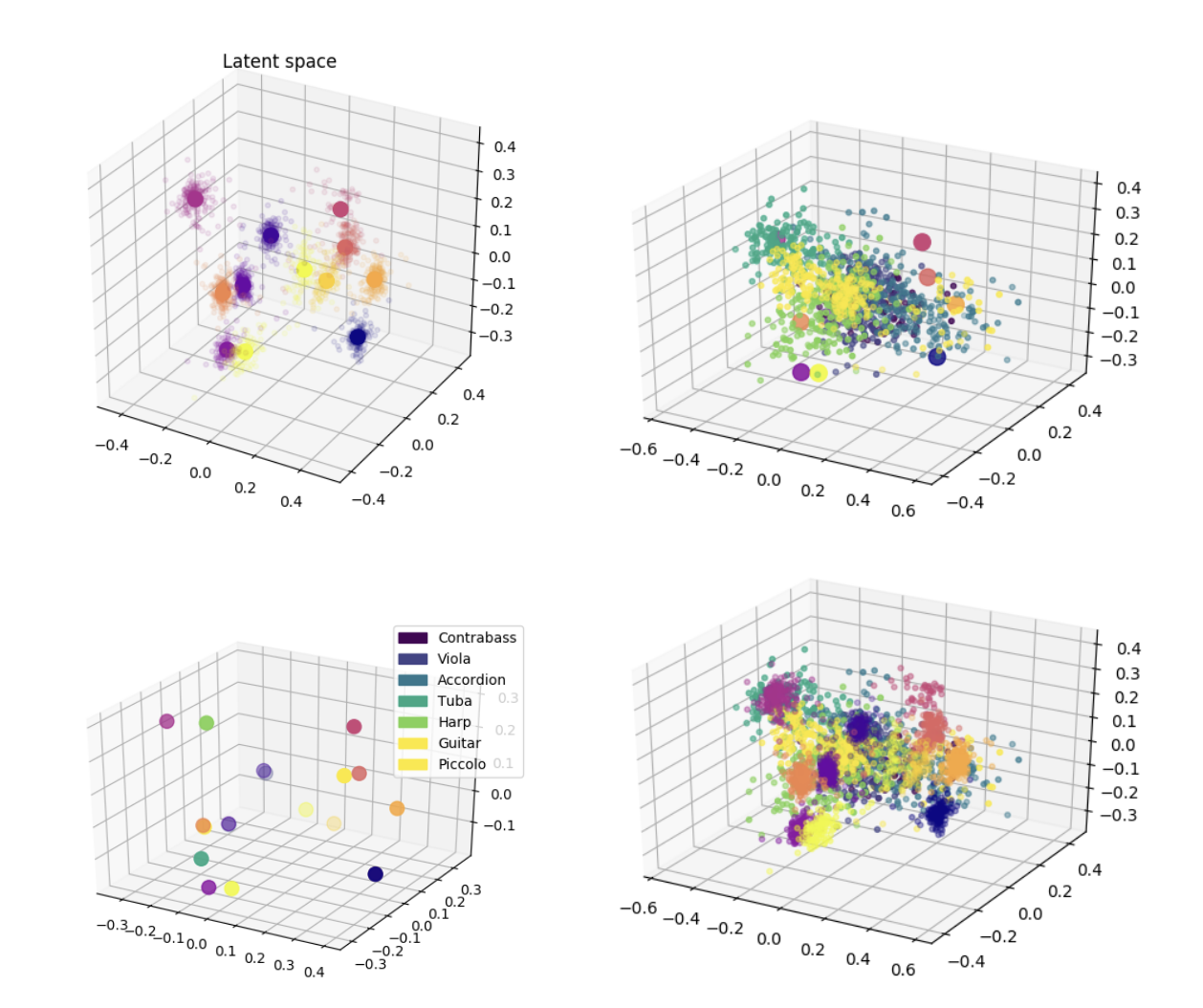
1. Pitch-Timbre Disentanglement Of Musical Instrument Sounds Based On Vae-Based Metric Learning - This paper modifies the VAE architecture slightly to better disentangle pitch and timbre. It uses contrastive loss functions to construct two latent spaces for pitch and timbre. Both losses are also weighted by hyperparameters.

As you can see below, their model does a much better job in the timbre space at creating separate clusters. Their change to the traditonal architecture is surprisingly effective for being so minimal.

1. Generative variational timbre spaces - This paper makes use of a traditional VAE, but regularizes the latent space with perceptual ratings. To improve disentanglement, a hyperparameter weight is attatched to the KL-Divergence term as well. The result is a very nice latent space, with some cool results from interpolating through.
2. WaveNet - I recommend reading this paper on your own as it’s really well written and groundbreaking in the field of time-series deep-learning. What makes WaveNet so unique is that it deals with raw audio signals with a modified Convolutional Neural Network, yet it still has better consistency and quality than other methods.

Future Work

Swapping VAE - There’s lots of potential in this project for timbre but it’s relatively unexplored. This suggests using two VAE-GANS. One VAE-GAN creates two separate latent spaces, one for the content of an image and the other for texture present in the image. Then, the 2048-dimensional latent vector is swapped with the latent vector for another VAE-GAN, transferring that style to the other. It’s a “plug and play” sort of architecture, and has incredible results across a wide array of scenes. I’d love to see – or implement – a swapping VAE architecture on an audio dataset.

Perceptual Ratings As Regularization - As is the case with the “Generative variational timbre spaces” paper cited before, this network includes a regularization parameter using perceptual ratings. While this does introduce a latent space regularization - reconstruction quality trade-off, it seems to be worth it because of the more intutitive latent space.

This article serves as a simple summary of the past research, current models, new architectures, and possible future solutions. I’ll continue to post updates on this project as I implement my own models. Right now, I’m looking into implementing the Swapping VAE. I’ve applied a vanilla and Beta-VAE. While Beta seems to perform better at disentanglement, both lack reconstruction quality. This is partly due to the limitations of Mel-spectrograms but also because of the model and data itself. As I curate a better dataset and get better audio samples, I’ll post those along with relevant snapshots of the latent space.