Disproving the Myth of “Positionless Basketball” with K-Means Clustering
“Positionless Basketball” is a misnomer. It’s no wonder that the standards created over half a century ago no longer apply to today’s game, and we shouldn’t expect them to. Bigs can shoot threes, point guards do more than pass, and some seven-footers pass like Magic. It’s time to change how we define NBA positions — Enter K-Means.
K-Means is an unsupervised machine learning algorithm that groups, or clusters, data together. It does this by randomly selecting some points, assigning other points to them based on distance, and then iteratively optimizing until it finds the best clusters. See here for a much more detailed explanation[1]. These groupings can give us insights into relationships we hadn’t previously known about.
With that, let’s begin:
Part 1: Collecting Data
There are a few ways to get the data we want, but all of them involve reaching endpoints in one way or another. An endpoint is where we access the data directly from a server. Here are the options for accessing data:
One is scraping player data from Basketball Reference. This is a good option if you want data from before the 1996–97 season(how far back the NBA’s site goes). Today, we don’t need anything but the 2020–21 season.
Another option is using NBA’s stat page. If you navigate to sortable player/team stats, that’s where you’ll find what you need. Clicking through the tabs will give you access to all their data, including some really advanced stuff like playtypes and tracking. These advanced stats are why I prefer using the NBA’s website, but there’s also the drawback that sometimes websites will block requests if you make too many. A good fix that I’ve learned is to throw a 3 second sleep into whatever you’re looping.
Lastly, you can use python libraries other people have created to “abstract away” the need to scrape. I don’t like using libraries because they can become outdated, and the visual tables on nba.com make it easier to find what I’m looking for. However, here are some excellent options:
nba_api— this is the most extensive API library for nba.com data, and it has documentation on all the endpoints. For info on how to use it, I recommend this article.py-goldsberry— named after the famous statmeister Kirk Goldsberry, this library also uses nba.com but is slightly easier to pick up in terms of syntax than nba_api, in my opinion.basketball_reference_scraper— as the name goes, this API gets the stats from Basketball Reference. Like author “Vishaala Gartha” says, using this has the advantage of being able to request large amounts of data without being blocked from requests.
Today, we’ll be manually scraping from nba.com since that’s my method of choice.
First, you have to find the data you want. Players — General — Traditional is the page for simple data like PTS, FG%, 3PA, REB, STL, etc. We want this basic data for our position classifier, but I’m using the 2020–21 season. Now, it’s not as easy copying the link; you have to do a little bit of digging. It might seem confusing at first, but it’s really not once you get it down.
Open up Developer Tools(ctrl-shift-I on Chrome and Windows), navigate to the network tab, and then refresh the page. You’ll see a bunch of complicated links under the Name tab, but what we’re looking for begins with leaguedashplayerstats(it’ll say this for every stat category). Sorting by name makes it easier to find, but make sure you get the one with type xhr if you see two. Copy the request URL.
This is what you’ll send the GET request to — make sure to install and import the package requests to get the data. We’re also going to be using pandas, so import that while you’re at it. Whenever requesting from nba.com, include these headers that allow the query to go through.
import requestsheaders  = {
    'Connection': 'keep-alive',
    'Accept': 'application/json, text/plain, */*',
    'x-nba-stats-token': 'true',
    'User-Agent': 'Mozilla/5.0 (Macintosh; Intel Mac OS X 10_14_6)       AppleWebKit/537.36 (KHTML, like Gecko) Chrome/79.0.3945.130 Safari/537.36',
    'x-nba-stats-origin': 'stats',
    'Sec-Fetch-Site': 'same-origin',
    'Sec-Fetch-Mode': 'cors',
    'Referer': 'https://stats.nba.com/',
    'Accept-Encoding': 'gzip, deflate, br',
    'Accept-Language': 'en-US,en;q=0.9',
}
basic_url = 'https://stats.nba.com/stats/leaguedashplayerstats?College=&Conference=&Country=&DateFrom=&DateTo=&Division=&DraftPick=&DraftYear=&GameScope=&GameSegment=&Height=&LastNGames=0&LeagueID=00&Location=&MeasureType=Base&Month=0&OpponentTeamID=0&Outcome=&PORound=0&PaceAdjust=N&PerMode=PerGame&Period=0&PlayerExperience=&PlayerPosition=&PlusMinus=N&Rank=N&Season=2020-21&SeasonSegment=&SeasonType=Regular+Season&ShotClockRange=&StarterBench=&TeamID=0&TwoWay=0&VsConference=&VsDivision=&Weight='
Now we make the request and use .json() to convert the request response object information into json data [2]:
json_basic = requests.get(basic_url,headers=headers).json()
If you look through the json data, you’ll notice that everything we want(stat categories and the data itself) is under [“resultSets”][0]. The features(e.g. PLAYER_NAME, FG%) come by [“headers”] and the data from [“rowSet”]. We have to convert the data to a pandas DataFrame so we can manipulate it better.
features = json_basic['resultSets'][0]['headers']
data = pd.DataFrame(json_basic['resultSets'][0]['rowSet'])data.columns = features
Notice that I set the columns of data = features, this makes the columns align with their actual name, instead of being ordered by [0,1,2,3,…]
Our “data” DataFrame should look like this now:
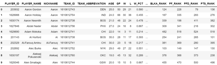
While this data can be useful, there’s a lot of junk. We’re gonna have to change that but for the time being take a second to think about which category could be useful for categorizing playtypes. Do we want it to discriminate based on wins or losses, or fantasy points, or nickname?
We’re going to leave that until later on to simplify things a little. For now, I think we need more data. Although these basic stats tell us something, it lacks the complexity that will help differentiate some different players from the others. Rebounding % actually gives us more information about a player’s rebounding ability than pure boards(Thinking Basketball explains this really well here). To get everything we want, let’s get some advanced data by using the same scraping technique on Players — General — Advanced. Lastly, I want to differentiate between inside scorers and perimeter shooters. Players — Shot Dashboard — General gives percentages based on distance. This gives us the following code in total(I wrapped the scraping process into a function because we have to repeat it multiple times):
import requestsheaders  = {
    'Connection': 'keep-alive',
    'Accept': 'application/json, text/plain, */*',
    'x-nba-stats-token': 'true',
    'User-Agent': 'Mozilla/5.0 (Macintosh; Intel Mac OS X 10_14_6)  AppleWebKit/537.36 (KHTML, like Gecko) Chrome/79.0.3945.130  Safari/537.36',
    'x-nba-stats-origin': 'stats',
    'Sec-Fetch-Site': 'same-origin',
    'Sec-Fetch-Mode': 'cors',
    'Referer': 'https://stats.nba.com/',
    'Accept-Encoding': 'gzip, deflate, br',
    'Accept-Language': 'en-US,en;q=0.9',
}basic_url = 'https://stats.nba.com/stats/leaguedashplayerstats?College=&Conference=&Country=&DateFrom=&DateTo=&Division=&DraftPick=&DraftYear=&GameScope=&GameSegment=&Height=&LastNGames=0&LeagueID=00&Location=&MeasureType=Base&Month=0&OpponentTeamID=0&Outcome=&PORound=0&PaceAdjust=N&PerMode=PerGame&Period=0&PlayerExperience=&PlayerPosition=&PlusMinus=N&Rank=N&Season=2020-21&SeasonSegment=&SeasonType=Regular+Season&ShotClockRange=&StarterBench=&TeamID=0&TwoWay=0&VsConference=&VsDivision=&Weight='advanced_url = 'https://stats.nba.com/stats/leaguedashplayerstats?College=&Conference=&Country=&DateFrom=&DateTo=&Division=&DraftPick=&DraftYear=&GameScope=&GameSegment=&Height=&LastNGames=0&LeagueID=00&Location=&MeasureType=Advanced&Month=0&OpponentTeamID=0&Outcome=&PORound=0&PaceAdjust=N&PerMode=PerGame&Period=0&PlayerExperience=&PlayerPosition=&PlusMinus=N&Rank=N&Season=2020-21&SeasonSegment=&SeasonType=Regular+Season&ShotClockRange=&StarterBench=&TeamID=0&TwoWay=0&VsConference=&VsDivision=&Weight='shotdash_url = 'https://stats.nba.com/stats/leaguedashplayerptshot?CloseDefDistRange=&College=&Conference=&Country=&DateFrom=&DateTo=&Division=&DraftPick=&DraftYear=&DribbleRange=&GameScope=&GameSegment=&GeneralRange=Overall&Height=&LastNGames=0&LeagueID=00&Location=&Month=0&OpponentTeamID=0&Outcome=&PORound=0&PaceAdjust=N&PerMode=PerGame&Period=0&PlayerExperience=&PlayerPosition=&PlusMinus=N&Rank=N&Season=2020-21&SeasonSegment=&SeasonType=Regular+Season&ShotClockRange=&ShotDistRange=&StarterBench=&TeamID=0&TouchTimeRange=&VsConference=&VsDivision=&Weight='

def get_data(url):
    json = requests.get(url,headers=headers).json()    features = json['resultSets'][0]['headers']
    data = pd.DataFrame(json['resultSets'][0]['rowSet'])    data.columns = features

    return datadata = get_data(basic_url)
advanced_data = get_data(advanced_url)
shotdash_data = get_data(shotdash_url)data_shotdash = data_shotdash[['PLAYER_NAME','FG2A_FREQUENCY', 'FG2M', 'FG2A', 'FG3A_FREQUENCY']]data_adv = data_adv[['PLAYER_NAME','USG_PCT','OFF_RATING','DEF_RATING','AST_PCT','AST_TO','AST_RATIO','OREB_PCT','REB_PCT','E_TOV_PCT','EFG_PCT','TS_PCT',]]
As you can see, I keep “PLAYER_NAME” each time. We want to aggregate this data into one DataFrame, but there has to be some common identifier. Names work well. Here’s how you combine them:
data = data.merge(data_adv,on='PLAYER_NAME')
data = data.merge(data_shotdash,on='PLAYER_NAME')
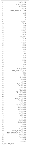
Data has 81 features, so let’s cut that down to the bare essentials. Immediately, we can take out everything non-stat-based, like player names, team names, age, or fantasy-related stats. We also want to remove players with less than 20 games played and 10 minutes since any with small sample sizes are “distorted.” There are also certain stats that we don’t want. Wins shouldn’t affect what group a player belongs to, for example. I’ll show what I took out below, but you should consider what will help the model perform better. I’m also gonna store the names in a DataFrame because we’ll want them later.
This is a quick way of eliminating all the rank-based stats that we don’t want in our model.
data.drop(data.filter(regex='RANK').columns, axis=1, inplace=True)data = data[(data['GP'] > 20) & (data['MIN'] > 10)]
names = data['PLAYER_NAME']data.drop(['PLAYER_NAME','W_PCT','PLAYER_ID','PFD','NICKNAME','TEAM_ID','TEAM_ABBREVIATION','AGE','GP','W','L','MIN','NBA_FANTASY_PTS','DD2','TD3','CFID','CFPARAMS', 'PLUS_MINUS','DREB'], axis=1, inplace=True)
The last step of the data part: scaling. You’ll want to import StandardScaler from sklearn.preprocessing. This standardizes by transforming the mean to 0 and the variance to 1. Standardizing is a necessary step before running PCA.
data = StandardScaler().fit_transform(data)
With all that out of the way, let’s get to the good part.
Part 2: Dimensionality Reduction with PCA
Principle Component Analysis(PCA) is a method for data visualization and dimensionality reduction that uses eigenvalues and some matrix algebra to calculate orthogonal components. Orthogonal means that these vectors are uncorrelated, so we’re getting the most info from the least components. These components will be ordered by explained variance, so the first component will “hold the most info.” If that didn’t make sense, just know that PCA is a way of squeezing our data down into a compressed form.
Dimensionality reduction helps in a few ways. For one, it cuts down on the cost of computation. Considering that we don’t lose much information when reducing all those features into 16 components, it’s a no-brainer. It also helps with visualization(as you’ll see in a second). Lastly, it avoids the problems with high-dimensional data like overfitting and other issues with the clustering algorithms. But don’t stress about that now, just know it’s a good practice.
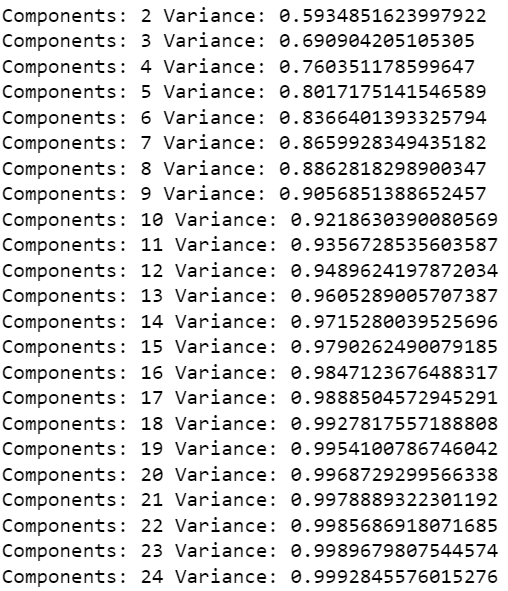
First, we want to figure out how many dimensions to actually reduce. There’s a tradeoff between achieving lower dimension data and keeping the information. Explained variance is a good way of measuring how much information we kept from the original to our PCA dataset. If you’ve ever taken a stats course, it’s really similar to R².
To get a good idea of the right number of principles components(which is like the number of features), lets run PCA at each component number and then calculate the explained variance for each of these.
from sklearn.decomposition import PCA
variances = []
for n_components in range(2,25):
    pca = PCA(n_components = n_components)
    components = pca.fit_transform(data)
    print('Components: {} Variance: {}'.format(n_components,         sum(pca.explained_variance_ratio_)))
    variances.append(sum(pca.explained_variance_ratio_))
Here we run fit_transform with our PCA model on each n_components from 2 to 25. Then, we sum the explained_variance_ratio_ to get the number we want since that’s the explained variance for each individual component.
This is what I got:
And the graph…
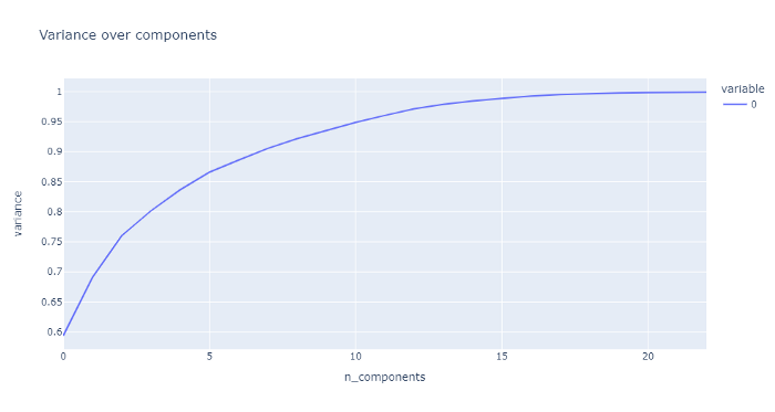
It approaches a horizontal asymptote, so we really lose the bang for our buck at a certain point. I’ll be going with 16 components.
pca = PCA(n_components=16)
components = pca.fit_transform(data)
Part 3: Running K-Means
We’ve got some nice looking, low dimensional, cleaned-up data that’s begging to be clustered. Thankfully, the process is somewhat similar to PCA in terms of syntax. We’re gonna create some metrics to judge the clustering(keeping in mind what we want to analyze).
Silhouette is a metric for evaluating the performance of clustering. It uses both intra-cluster distances(between points in a cluster) and inter-cluster distances(between clusters). 1 means a perfect cluster, while anything closer to 0 shows more and more overlap. -1 means you’ve got some error with samples in the cluster, but that shouldn’t be an issue. Inertia is another measurement that uses the distance from points to its centroid.
Using these two measurements, we should get a good idea of how many clusters to use.
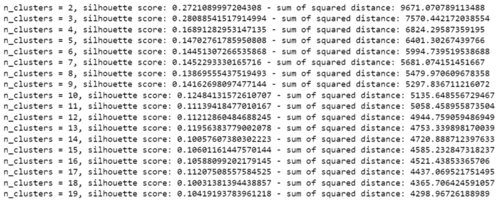
from sklearn.cluster import KMeans
from sklearn.metrics import silhouette_scoresilhouettes = []
sse = []
for n_clusters in range(2,20):

    kmeans = KMeans(n_clusters=n_clusters,random_state=84)

    cluster_labels = kmeans.fit_predict(components)

    silhouette = silhouette_score(components, cluster_labels)
    silhouettes.append(silhouette)
    sse.append(kmeans.inertia_)    print("n_clusters = {}, silhouette score: {} - sum of squared  distance: {}".format(n_clusters, silhouette, kmeans.inertia_))
Outcome:
Graphs:
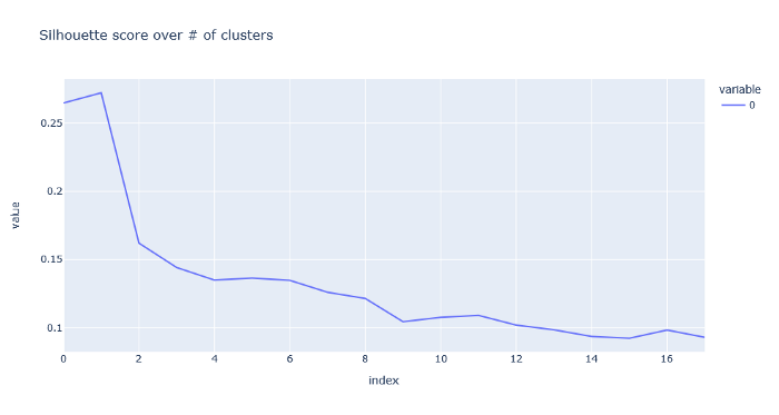
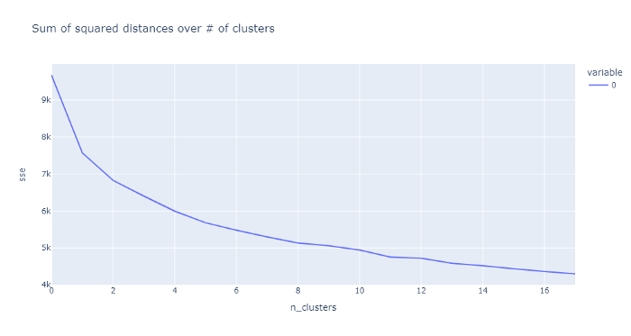
Don’t get too excited about these numbers. We obviously don’t want one or two clusters, so the high scores doesn’t mean anything to us. We also don’t want too many clusters since the effectiveness of the clusters seem to drop off quite a bit. 11 looks like a sweet spot.
We’re on the home stretch now. Since we know that 11 is a good number, all we have to do is run K-Means again.
kmeans = KMeans(n_clusters=11,random_state=42)kmeans.fit(components)
km = kmeans.predict(components)
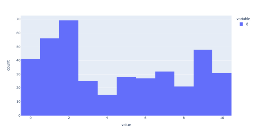
This is the distribution of clusters. We’ve got lots of twos and fives. It’s time to examine the clusters a long the data to see what it means. This is the really fun part.
Part 4: Cluster Analysis
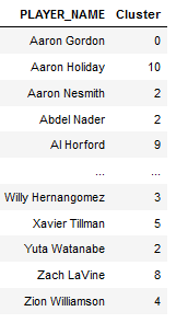
I want to organize this into a neat DataFrame and put the cluster groups alongisde players. It’ll make everything a lot easier to see.
final = pd.DataFrame()
final['PLAYER_NAME'] = names
final['Cluster'] = km
It should look something like this:
A cool way of visualizing the clustering algorithm is to graph the clusters along the first two PCA components — like so:
#Getting unique labels
label = km
u_labels = np.unique(label)
centroids = kmeans.cluster_centers_#plotting the results:
for i in u_labels:
    plt.scatter(components[label == i , 0] , components[label == i , 1] , label = i)
plt.scatter(centroids[:,0] , centroids[:,1] , s = 40, color = 'k')
plt.legend()
plt.show()
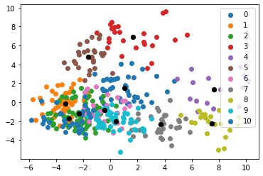
Hmm, doesn’t look great…
Although we could make changes to achieve more separate clustering, this graph sheds some light on the positionless basketball theory.
Playstyles are more fluid than they ever have been, so lots of players exist on the continuum somewhere in between. Clusters 3, 8, and 4 really stand out.
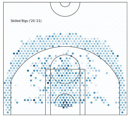
Cluster 0 — Skilled Bigs:
Here are the skilled, stretch-four type big men. Unlike the classic bigs who wouldn’t dare step outside the paint, these players represent the new era where bigs are encouraged to take the threes that are left open.
PTS: +1.6219015701607393 from average
USG_PCT: +0.013398622230497176 from average
E_TOV_PCT: -0.20089368832619492 from average
FG3A_FREQUENCY: -0.06461211444175508 from average
OFF_RATING: -0.6336684664556458 from average
DEF_RATING: +0.7761310742878322 from average
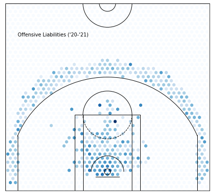
Cluster 1 —Offensive Liabilities :
 Sorry…
Not much needs to be said here, all these guys aren’t very good. To their credit, most are young or old.
PTS: -5.726617593602327 from average
OFF_RATING: -4.706752090149038 from average
DEF_RATING: +0.783056161395848 from average
TS_PCT: -0.05806302253725937 from average
Yikes, look at that efficiency.
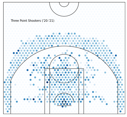
Cluster 2 —Three Point Shooters :
It’s pretty obvious what we’re looking at here: three-point specialists. Joe Harris, Joe Ingles, JJ Redick. These players should have a higher frequency of three-point shots in comparison to other players, as well as higher efficiency. Looking at volume will be misleading because the star guards will easily beat out these guys.
FG3A_FREQUENCY:+0.22087321606372384 from average
FG3_PCT: +0.06679156986392298 from average
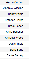
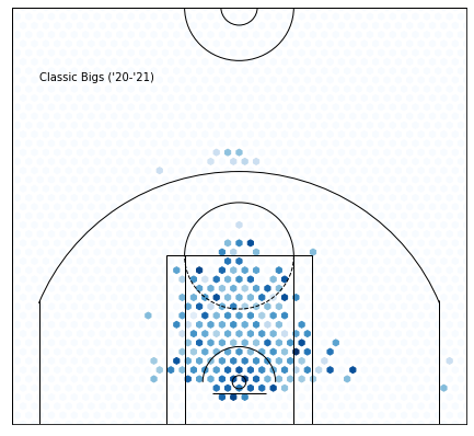
Cluster 3—Classic Bigs :
This is the only category that’s stuck since the classic positions were invented. The big-man’s responsibilities are to grab boards, be efficient(besides FT), and, whatever it takes, never take a three-pointer.
EFG_PCT: +0.07113903307888048 from average
OREB_PCT: +0.07840447837150125 from average
FG3A_FREQUENCY: -0.3746004071246819 from average
Notice the three-pointers from right at the top of the key — classic.
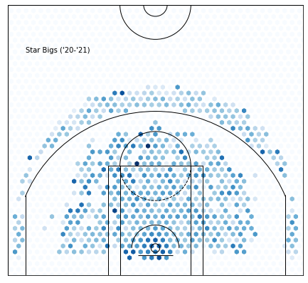
Cluster 4—Star Bigs :
It’s clear that this cluster is selecting for star bigs. Unlike star guards, who they share the most in common with, these players should have higher rebounding percentage, lower assist numbers, and better efficiency(besides free throws).
Side-note: Isn’t it weird that Jokic is here? I thought he’d be more “guard-y”.
AST_PCT: +0.12610839694656487 from average
OFF_RATING: +3.3401526717557317 from average
USG_PCT: +0.09076284987277355 from average
EFG_PCT: +0.00812569974554711 from average
OREB_PCT: +0.0172178117048346 from average
REB_PCT: +0.04435674300254451 from average
FGA: +7.756895674300255 from average
Hm, they’re not that much more efficient and rebounding isn’t that impressive. Also, what’s up with those passing numbers? Even their assist percentage to usage rate is high(you’ll figure out what this means later on), which says that star bigs really are decent at playmaking.
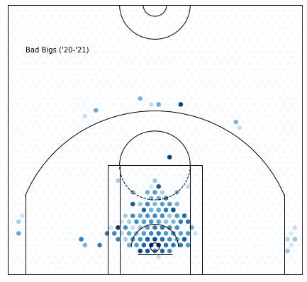
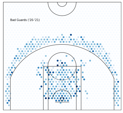
Cluster 5 —Bad Bigs :
These players are similar to the classic bigs in their skillset; they’re worse.
Image by Thomas Spangler on Wikimedia Commons
EFG_PCT: +0.06151617593602343 from average
OREB_PCT: +0.0518630498000727 from average
FG3A_FREQUENCY: -0.33127326426753906 from average
Everything is looking good here, but they separate from cluster 3 in volume.
PTS: -5.015903307888041 from average
REB: +0.1503089785532543 from average
OFF_RATING: -1.896037804434755 from average
DEF_RATING: -1.5258724100327186 from average
The defensive rating shows why these guys are still getting paid. Like the cluster 10 guards, they have a really good defensive rating that makes them almost positive in net rating.
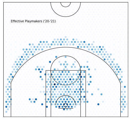
Cluster 6 —Effective Playmakers :
Rubio and Rondo make me think that we’re looking at playmakers here.
Image by Keith Allison on Wikimedia Commons
In particular, low volume, effective playmakers. This means that, while they don’t control the ball on that many possessions, they can create a lot of offense. Usage Rate(the percent of plays that a player uses) is a decent representation of volume. Assist percentage(the percent of field goals a player assists when they’re on the floor) is a good metric for playmaker effectiveness.
Dividing assist percentage by usage rate will give us a good idea of whether or not our suspision is right:
Cluster: 0 - ASSIST TO USAGE PCT: 0.4795830778663396
Cluster: 1 - ASSIST TO USAGE PCT: 0.6552994296577946
Cluster: 2 - ASSIST TO USAGE PCT: 0.6000000000000001
Cluster: 3 - ASSIST TO USAGE PCT: 0.5561824165491301
Cluster: 4 - ASSIST TO USAGE PCT: 0.9732142857142857
Cluster: 5 - ASSIST TO USAGE PCT: 0.5202834799608993
Cluster: 6 - ASSIST TO USAGE PCT: 1.3574868651488619
Cluster: 7 - ASSIST TO USAGE PCT: 1.029279568511622
Cluster: 8 - ASSIST TO USAGE PCT: 0.9058823529411765
Cluster: 9 - ASSIST TO USAGE PCT: 0.6472417251755265
Cluster: 10 - ASSIST TO USAGE PCT: 1.140148392415499
6 clearly stands out.
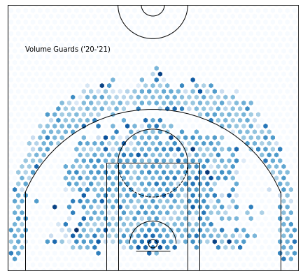
Cluster 7 —Volume Guards :
All these players are really good, but not quite at the cluster 8 level(besides CP3). I expect to see high total numbers at the cost of lower efficiency — ehem, Cole Anthony.
PTS: +6.82159669211196 from average
AST_PCT: +0.10771048027989824 from average
DEF_RATING: +0.6201097328244174 from average
USG_PCT: +0.05783993320610689 from average
TS_PCT: -0.014888915394402069 from average
FGA: +6.040020674300253 from average
I wouldn’t be too suprised by the high assist percentage. We’re comparing with the rest of the league, so no wonder high usage-rate guards are gonna be assisting a lot.
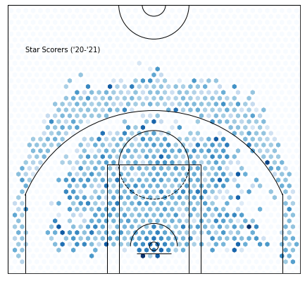
Cluster 8 —Star Scorers:
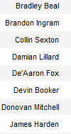
This cluster is clearly showing star guards. I’m expecting high offensive productivity with high volume.
PTS: +15.053144311159578 from average
AST: +3.443475099963651 from average
OFF_RATING: +5.5230098146128626 from average
USG_PCT: +0.1180676117775355 from average
TS_PCT: +0.03465721555797874 from average
FGA: +10.294038531443112 from average
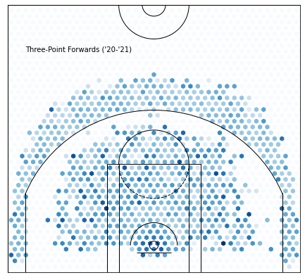
Cluster 9 —Three Point Forwards:
Image by David Shankbone on Wikimedia Commons
It’s interesting that K-Means was able to pick up on differences between three point shooting guards and forwards, since the statistical differences are minor.
3PT Forwards:
PTS: +2.4590966921119612 from average
FGA: +2.3660623409669217 from average
AST_PCT: -0.00832076972010179 from average
FG3A_FREQUENCY: +0.10482792620865139 from average
FG3A: +2.1830629770992362 from average
FG3_PCT: +0.04487309160305347 from average
USG_PCT: +0.02220451653944025 from average
EFG_PCT: -0.01050763358778617 from average
3PT Guards:
PTS: -2.8659033078880416 from average
FGA: -2.3254231662794567 from average
AST_PCT: -0.05328000885053655 from average
FG3A_FREQUENCY: +0.22087321606372384 from average
FG3A: +0.5690231220267727 from average
FG3_PCT: +0.06679156986392298 from average
USG_PCT: -0.0363733820112844 from average
EFG_PCT: +0.033630047571634125 from average
This tells us that the guard category is much more specialized in what they do than forwards. Forwards score four more points on average and take significantly more shots, but guards shoot more threes in total. They’re also less active playmakers and hold the ball less.
Cluster 10—Low Volume… Low efficiency…Good Defense???:
Even though we select players with over 10 minutes per game, we still get a lot of players who have very low volume and efficiency. This seems strange since most teams don’t want this type of player on their team, but I think this inadvertently selects for skilled defenders. The players who don’t have great offensive stats and still get minutes must be solid defenders, or otherwise, they wouldn’t be on the floor that much. Interestingly, their -2.94 Offensive Rating is nearly compensated by their high defensive rating.
PTS: -5.349774275629977 from average
OFF_RATING: -2.943503242222775 from average
DEF_RATING: -2.7031765574981534 from average
TS_PCT: -0.06265000410407962 from average
Observations:
If we attach the net rating of a player’s team to their cluster and then take the average net rating for each cluster, it might give an idea of how rosters are constructed and what players help them perform well.
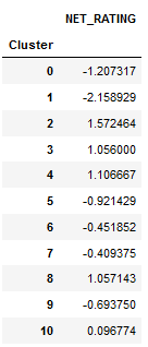
As you can see, offensive liabilities(cluster 1) tend to be on bad teams. Teams that play 1-ers for more than ten minutes a night are probably either tanking or simply lack a good roster. On the other hand, three-point shooters usually seem to be on very good teams. The teams that rely on three-point shooters, like Utah, are generally very efficient and have high offensive ratings. Keep in mind that net rating is subject to some biases in the way it’s calculated.
General Conclusions:
Admittedly, I wouldn’t call some of these clusters positions. Positions are supposed to be based on playstyle, not volume or efficiency. The players with high usage rates don’t seem to perform as well with clustering since they excel in every stat and therefore are “inflated,” but this could likely be compensated for using adjusted stats(like per possession).
Future Ideas:
You can do a lot using this basic method of clustering data. Applying K-Means to team stats instead could tell you which team playstyles tend to perform well. If you use the same clusters but predict earlier seasons, you could see how certain platypes have grown or decreased in popularity over time(like 3 point shooters). Maybe you find the perfect roster by tracking how a team’s success correlates to the distribution of their clusters — this could come in handy for fantasy. The moral of the story is that you should try experimenting with this on some new data and see what you get.
References:
[1] J. Starmer, StatQuest: K-means clustering(2018), https://www.youtube.com/watch?v=4b5d3muPQmA
[2] W3 School, Python requests.Response Object, https://www.youtube.com/watch?v=4b5d3muPQmA